3.4. Linear Regression Implementation from Scratch — Dive into Deep Learning 1.0.3 documentation
d2l.ai
[1]
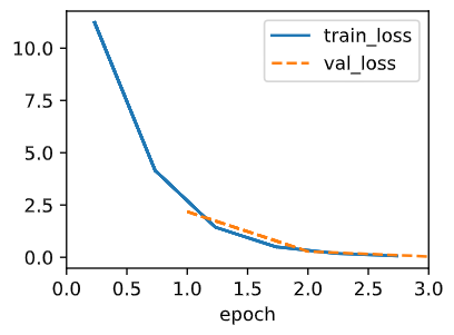
The algorithm will still work even if the weight is initially zero. Since the algorithm we are using is gradient descent, typically it doesn't matter where you start. The gradient will mostly always guide the weight to the spot where the loss function is minimum. We can confirm this by running the code from the book after changing the weight to `torch.zeros`.
self.w = torch.zeros((num_inputs, 1), requires_grad=True) # only changed coderesult >>

The variance doesn't even matter since we can initialize the weight to whatever we want. Since the gradient descent algorithm will always guide us to the global minima. One thing to note is that when the variance is large, the initial weight will be big, resulting in a huge loss at the beginning of the training session.

[2]
Since we want to predict the resistence(R) given voltage(V) and current(I), we have to solve the equation
$V=w_{1}*I+b$. This in only worth the try if Ohm plotted V and I and noticed the linear correlation between those two features. If we run the model for V and I, which can be achieved from a resister, b would be 0 and $w_{1}$ will equal to R.
[3]
Let's first make things clear; we want to predict the temperature. However, unlike most other regressions we did, temperature is not the target variable. The target variable is actually $B(\lambda, T)$ and the feature variable is $\lambda$. $T$ will only take part as a parameter.
For convenience $\lambda$ will be X, $B(\lambda, T)$ will be y, $T$ will be just t in the code.
We just have to make little adjustment to the already written code.
- Make a new function for the model based on the Plank equation.
- self.X should be a continuous value. Since X will be the wavelength like the picture below. Also Plank equation handles very small units thus we have to shurink the data that are generated by the torch library(such as X and noise).

final code >>
from d2l import torch as d2l
import matplotlib.pyplot as plt
import torch
def f(t, x):
    c = 299792458
    h = 6.6260701e-34
    k = 1.380649e-23
    beta = h*c/(k*x)
    alpha = 2*h*c**2/x**5
    return alpha/(torch.exp(beta/t)-1)

class SyntheticPlankData(d2l.DataModule):
    def __init__(self, T, noise=0.05, num_train=1000, num_val=1000,
                batch_size=32):
        super().__init__()
        self.save_hyperparameters()
        n=num_train+num_val
        self.X=torch.arange(300, 300+n)*1e-9
        noise=torch.randn(n, 1)*noise
        self.y=f(t, self.X)+noise.reshape((n,))


    def get_tensorloader(self, tensor, train, indices=slice(0, None)):
        tensor = tuple(a[indices] for a in tensor)
        dataset = torch.utils.data.TensorDataset(*tensor)
        return torch.utils.data.DataLoader(dataset, self.batch_size,
                                            shuffle=train)

    def get_dataloader(self, train):
        i = slice(0, self.num_train) if train else slice(self.num_train, None)
        return self.get_tensorloader((self.X, self.y), train, i)

class PlankModel(d2l.Module):
    def __init__(self, t=0, lr=1e-21, sigma=0.01):
        super().__init__()
        self.save_hyperparameters()
        self.t = torch.Tensor([t])
        self.t.requires_grad = True

    def forward(self, X):
        return f(self.t, X)

    def loss(self, y_hat, y):
        l = (y_hat-y)**2/2
        return l.mean()

    def configure_optimizers(self):
        return d2l.SGD([self.t], self.lr)
# drawing the data
T=[2000, 4000, 5000]
ls=[]
for t in T:
    ls.append(SyntheticPlankData(t))
    plt.scatter(ls[-1].X, ls[-1].y, label=t, alpha=0.3)
plt.legend()
plt.show()
data=SyntheticPlankData(5000)
model=PlankModel(t=3000)
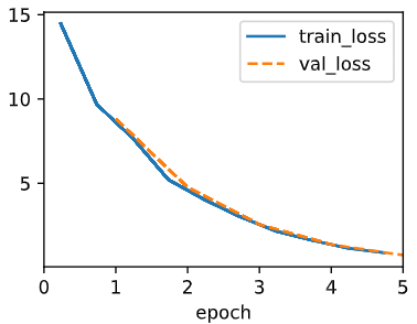
trainer=d2l.Trainer(max_epochs=5)
trainer.fit(model, data)
print(model.t)
[4]
If you run this simple code for integrating twice,
import torch
def loss(y_hat, y):
    l = (y_hat - y.reshape(y_hat.shape))**2/2
    return l.mean()

x = torch.tensor([[1., 2.]]) # 1*2
b = torch.tensor([1.]).requires_grad_(True)
w = torch.tensor([1.,2.]).reshape(-1,1).requires_grad_(True) # 2*1
y_hat = (torch.matmul(x, w) + b)
y = torch.tensor([5.])
loss = loss(y_hat, y)
loss.backward()
print(w.grad, b.grad)
loss.backward()
print(w.grad, b.grad)
You will get this error message.
"RuntimeError: Trying to backward through the graph a second time (or directly access saved tensors after they have already been freed). Saved intermediate values of the graph are freed when you call .backward() or autograd.grad(). Specify retain_graph=True if you need to backward through the graph a second time or if you need to access saved tensors after calling backward."
Thus we need to add retain_graph=True to the loss.backward()
[5]
It may be used when elemenwise operation is needed.
[6]
Let's try multiple learning rates step by step. For unity, epoch will always be 5.
We will also look at the difference between predicted weights and the real weights by the following code.
print(f"weight diff = {abs(data.w.reshape(1, -1)-model.w.reshape(1, -1))}\nbias diff = {abs(data.b-model.b)}")
1. lr=2
This part was very interesting because some attepts showed good prediction while others were terrible.

In this case, the loss exploded and went to a gradual hault. And the differences from the correct w and b are not that bad


Every condition is the same as above, but the loss became huge and the diff got much bigger

This is because the learning rate is too big resulting in divergence around the global minima. The fun thing is that if we increase the epoch to 50, the loss calms down a bit, but not always.

2.lr=0.1


It became much better in the perspective of outcome and stability compared to lr=2. Another fun thing is that it seems to find the exact bulls eye in one go.
3. lr=0.01


It still has pretty decent performance but the speed became much slower. We can fix this problem by increasing the epoch so to give more time for the weights to find the global minima
4. lr=0.001


It becomes incredibly slow after 0.01.
Thus we learned that there is a specific point in the learning rate where it is most fast at lowering the loss. Also bigger epoch will guarantee better parameters, but has a cost(longer time).
[7]
We already saw the process with leftover batch in 3.3.5
[8-1]

It seems MAE is better than MSE. MAE doesn't square the loss, thus it is much more stable. The absolute value gives equal panalties proportionally to the difference.
[8-2]
What wil happen if we change data.y[5] to 10000? thus making it an outlier data.
model = LinearRegressionScratch(2, lr=0.01, sigma=0.01)
data = d2l.SyntheticRegressionData(w=torch.tensor([2, -3.4]), b=4.2)
data.y[5]=10000
trainer = d2l.Trainer(max_epochs=5)
trainer.fit(model, data) # the fit method calls the fit_epoch method
Despite the fluctuation of train_loss, parameters came out quite decent. The impact of daata.y[5] being 10000 is a considerable impact on the training set bacause values of y are mostly under 10. Also machine learning models are highly ruled by statistical assumptions and having an outlier data might violate that particular assumption. In the case of liner regression, noise of the data is thought to follow the gaussian distribution.

Fun thing is if I change the code like this
model = LinearRegressionScratch(2, lr=0.01, sigma=0.01)
data = d2l.SyntheticRegressionData(w=torch.tensor([2, -3.4]), b=4.2)
data.y[1005]=10000
trainer = d2l.Trainer(max_epochs=5)
trainer.fit(model, data) # the fit method calls the fit_epoch method
Another thing to note is that MSE is more affected by the outlier than MAE.


This can be explained in the perspective of whon each model chooses to focus. MSE impose huge penalties to outlier data since it squares the difference. On the other hand, as I mentioned earlier, penalty is imposed linearly to the magnitude of the difference.
[8-3]
We can achieve the partial benefits from both loss functions by using Huber loss.
ls=[] # to track the frequency
@d2l.add_to_class(LinearRegressionScratch)  #@save
def loss(self, y_hat, y, threshold=100):
    """
    returns the loss, which is represented as a n*1 tensor.
    """
    if abs(y_hat - y).sum()<threshold:
        ls.append("MSE")
        l = (y_hat - y)**2/2
    else:
        ls.append("MAE")
        l = (y_hat - y).abs().sum()
    return l.mean()
....
model = LinearRegressionScratch(2, lr=0.01, sigma=0.01)
data = d2l.SyntheticRegressionData(w=torch.tensor([2, -3.4]), b=4.2)
data.y[5]=10000
trainer = d2l.Trainer(max_epochs=5)
trainer.fit(model, data) # the fit method calls the fit_epoch method
print(ls.count("MAE"), ls.count("MSE"))


Warning : the equation does not actually correspond to Huber loss.
Even with bigger outliers for data.y[5], the model still stayed ontrack and showed small parameter difference.
[9]
Reshuffle is needed for the training process because certain data's might be clusterd only in the training set which will lead the model to memorize cases. It is dangerous since it can lead to overfitting or data leak. Also randomizing the data will make the results of validation data to be more reliable.
'ML&DL > Dive into Deep Learning' 카테고리의 다른 글
| [3.6.5] Dive into Deep Learning : exercise answers (0) | 2024.02.15 |
|---|---|
| [3.5.6] Dive into Deep Learning : exercise answers (1) | 2024.02.12 |
| [3.3.5] Dive into Deep Learning : exercise answers (0) | 2024.02.10 |
| [3.2.6]Dive into Deep Learning : exercise answers (0) | 2024.02.09 |
| [3.1.6]Dive into Deep Learning : exercise answers (1) | 2024.01.28 |

