3.5. Concise Implementation of Linear Regression — Dive into Deep Learning 1.0.3 documentation
d2l.ai
[1]
Let's say that the original loss function returns the total sum of the batch's loss(the learning rate is α and batch size is n). Thus the total impact of the loss will be α×loss(y_hat,y). However if we want the loss function to return the mean of the summed loss(loss′(y_hat,y)), in order to match the same influence from above, the total will be nα×loss′(y_hat,y). Thus we have to adjust the learning rate to α:=nα
[2]
The given equation is the Smooth L1 loss. However it will be halpful if we also look at the Huber loss.
@d2l.add_to_class(LinearRegression)  #@save
def loss(self, y_hat, y):
    # fn = nn.SmoothL1Loss()
    # fn = nn.HuberLoss()
    return fn(y_hat, y) # Use either loss function
....
model = LinearRegression(lr=0.03)
data = d2l.SyntheticRegressionData(w=torch.tensor([2, -3.4]), b=4.2)
data.y[[range(10)]]=10000 # 10 outliers
trainer = d2l.Trainer(max_epochs=10)
trainer.fit(model, data)

def get_w_b(self):
    return (self.net.weight.data, self.net.bias.data)
w, b = model.get_w_b()

print(f'error in estimating w: {abs(data.w - w.reshape(data.w.shape))}')
print(f'error in estimating b: {abs(data.b - b)}')


It seems that Huber and SmoothL1 are more robust than MSE for when outlier data's are in the dataset.
[3]
Use this code to see the grad of the model.
model.net.weight.grad
Here is the way to check the grad. Gradients are affected by the returned value of the loss function.


The grad has increased about 10 times compared to the original loss return. Through this step we can see if model.net.weight.grad is actually pointing to the grad of the model.
[4]
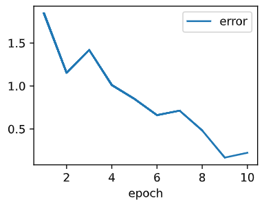
Let's first see how error of the first weight change through epoch=1 ~ epoch 10.
We will use this changes in code.
epoch_track = []
@d2l.add_to_class(LinearRegression)  #@save
def get_w_b(self):
	return (self.net.weight.data, self.net.bias.data)
for i in range(1, 11):
    model = LinearRegression(lr=0.03)
    data = d2l.SyntheticRegressionData(w=torch.tensor([2, -3.4]), b=4.2)
    trainer = d2l.Trainer(max_epochs=i)
    trainer.fit(model, data)

    w, b = model.get_w_b()
    epoch_track.append(data.w[0] - w.reshape(data.w.shape)[0])
....
board = d2l.ProgressBoard('epoch')
for x in range(1, 11):
    board.draw(x, epoch_track[x-1], 'error', every_n=1)
1. lr=0.03

More epoch doesn't neccesarily decrease the error, rather it diverges around 0.000.
2. lr=0.003

Significantly the bigger epoch gaurantee smaller error. From our experience, the learning rate preforms best when it is 0.03
3. lr=0.0003

As we can see that bigger epoch does help in decreasing errors but not always.
[5-1]
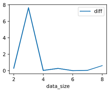
We must modify the code
data_track = []
@d2l.add_to_class(LinearRegression)  #@save
def get_w_b(self):
    return (self.net.weight.data, self.net.bias.data)
for i in range(2, 11):
    model = LinearRegression(lr=0.03)
    data = d2l.SyntheticRegressionData(w=torch.tensor([2, -3.4]), b=4.2, num_train=int(torch.log2(torch.tensor([100*i]))), num_val=int(torch.log2(torch.tensor([100*i]))))
    trainer = d2l.Trainer(max_epochs=5)
    trainer.fit(model, data)
    w, b = model.get_w_b()
    data_track.append(data.w[0] - w.reshape(data.w.shape)[0])
....
board = d2l.ProgressBoard('data_size')
for x in range(2, 9):
    board.draw(x, abs(data_track[x-2]), 'diff', every_n=1)

[5-2]
I really can't figure out the reason, so I this is the Gemini's answere to the question.
1. Efficiency: Training on the entire dataset can be computationally expensive, especially for large datasets. Logarithmic increases allow you to explore a wider range of data sizes while making more efficient use of your resources. By doubling the data size each time, you can cover a broader range of data sizes with fewer training runs compared to linear increases.
2. Diminishing returns: The performance gains from additional data often diminish as the data size increases. Logarithmic increases help you observe this phenomenon more clearly. As you double the data size, the performance improvement tends to become smaller and smaller, allowing you to identify the point where adding more data doesn't significantly improve the model anymore.
3. Practicality: Datasets often have natural logarithmic structures. For example, the number of users on a social media platform might grow exponentially at first, but eventually, the growth slows down and follows a more logarithmic pattern. Using logarithmic increases reflects this real-world distribution of data sizes.
4. Better visualization: Plotting performance against data size on a logarithmic scale can help visualize the trends more clearly. This is because a logarithmic scale stretches out the smaller data sizes, allowing you to discern subtle changes in performance at lower data regimes.
'ML&DL > Dive into Deep Learning' 카테고리의 다른 글
| [3.7.6] Dive into Deep Learning : exercise answers (1) | 2024.02.15 |
|---|---|
| [3.6.5] Dive into Deep Learning : exercise answers (0) | 2024.02.15 |
| [3.4.6] Dive into Deep Learning : exercise answers (1) | 2024.02.11 |
| [3.3.5] Dive into Deep Learning : exercise answers (0) | 2024.02.10 |
| [3.2.6]Dive into Deep Learning : exercise answers (0) | 2024.02.09 |


